Episodic Decision Problem

Definition. An episodic decision problem is defined by the following:

1. An action space $A$.
2. A reward function class $\c{R} \subseteq \{r : A\to\R\}$.
3. One of the following forms of ground-truth rewards:
   1. A true reward function $r\in\c{R}$.
   2. A reward distribution $q\in\c{M}_1(\c{R})$.
   3. A sequence of true reward functions $r_t\in\c{R}$ for $t=1,..,T$.
4. An observation space $\Sigma$.
5. A feedback function $\sigma : \c{R} \x A \to \c{M}_1(\Sigma)$.

Example: Black-box Optimization

Example. An episodic decision problem is called black-box optimization if:

1. The action space is $A = [0,1]^d$.
2. The reward function class is $\c{R}\subseteq \htmlClass{anchor-1}{C(A;\R)}$.
3. Examples from this talk: stochastic variant.
4. The observation space is $\Sigma=\R$.
5. The feedback function is $\sigma(r,a)=r(a)$, without any noise.

Bayesian optimization: black-box optimization using Bayesian algorithms

Bayesian Optimization

Automatic explore-exploit tradeoff

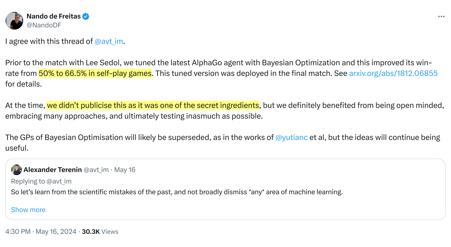
Performance Impact

Algorithms for Decision-making

An algorithm is a function $p : \htmlClass{anchor-1}{\f{Seq}(A \x \Sigma)} \to \htmlClass{anchor-2}{\c{M}_1(A)}$.

A Bayesian algorithm is a pair consisting of:

1. A Bayesian model, represented by posterior $\htmlClass{anchor-5}{p_{r\given a_{1:t},\sigma_{1:t}}}$.
2. A decision rule $\delta : \htmlClass{anchor-3}{\c{M}_1(\c{R})} \to \htmlClass{anchor-4}{\c{M}_1(A)}$.

What does it mean for an algorithm to perform well?

Regret

Stochastic variant: $$ R_T(p, r) = \E_{a_t\~p} \htmlClass{anchor-1}{\sup_{a\in A} \sum_{t=1}^{\smash{T}} r(a)} - \htmlClass{anchor-2}{\sum_{t=1}^{\smash{T}} r(a_t)} $$

reward under optimal action

total reward of learner's actions

Difference between rewards obtained, and what would have been obtained if there were no uncertainty

Other problem variants: slightly different notion of regret

example: Bayesian variant

average over $r\~q$

A Few Simple Algorithms

gap between averageand best point, nolearning, over-explores

can equal the worstpossible regret, nolearning or exploration

learns correctly but explorestoo little and can get stuckin suboptimal actions

What's missing from these? Balance between explore and exploit

Problem Difficulty

We don't know $r$, just that $r\in\c{R}$. What regret is even possible?

• Challenge: if we ask what is possible, then $p$ can do anything
• Approach: consider randomized problems

many strong algorithms:very different-lookingdesign principles

$R_T(p,r) \leadsto R_T(p,q)$

Lemma. Suppose there is a $q\in\c{M}_1(\c{R})$ such that, for any $p\in\c{P}$, we have $C \leq \E_{r\~q} R_T(p,r)$. Then for every $p\in\c{P}$ there is an $r_p\in\c{R}$ for which $C \leq R_T(p,r_p)$.

Hard distribution implies existence of hard instance

Lower Bounds

How do we find hard distributions?

• Idea: randomize over rewards that are different, but look the same

in a balanced manner so thelearner can't predict from $q$ alone

actions good for onereward are bad for others

hard to tell differentreward functions apart

Proposition. Consider a stochastic multi-armed bandit, with bounded rewards $\c{R} = \{r : A \to [0,1]\}$ and standard Gaussian noise. Define the reward distribution $q$ according to $$ \htmlData{class=fragment,fragment-index=14}{ r(a) } \htmlData{class=fragment,fragment-index=15}{ = } \htmlData{class=fragment,fragment-index=16}{ \begin{cases} \htmlData{class=fragment,fragment-index=17}{ \Delta } & \htmlData{class=fragment,fragment-index=18}{ a=\alpha } \\ \htmlData{class=fragment,fragment-index=19}{ 0 } & \htmlData{class=fragment,fragment-index=20}{ a\neq\alpha } \end{cases} } \qquad\qquad\qquad \htmlData{class=fragment,fragment-index=21}{ \alpha \~ \f{U}(A) . } $$ Under this distribution, if $K = |A| \geq 2$ and $T \geq \frac{K}{4}$, and $\Delta = \frac{1}{2}\sqrt{\frac{K}{T}}$, then we have $\frac{1}{8}\sqrt{KT} \leq R_T(\., q)$.

Bayesian Decision-making Algorithms

Many possible design principles:

• Expected improvement: approximate dynamic programming
• Gittins index: compare using equivalent fair value
• Optimism: pretend that best realistic world is correct
• Information-theoretic: pick points that provide information
• Thompson sampling: explore by random actions

Each approach: resolves uncertainty provided by the model differently

Thompson Sampling

Same model, different decisions, similar performance

Large Language Models

LLMs can solve episodic decision problems defined in token space

• Exploration principle: random sampling from softmax scores

some form of Thompson sampling?

Works in practice, even under partial feedback

• Open problem: understand why
• Challenge: one can show that naïve Thompson sampling can be bad

the problem: Thompson sampling never pickslow-reward-but-informative points

My view: promising direction for understanding how LLMs work